
Given the limits on time, attention and resources with which every cyber team must contend, risk assessment plays a critical role in helping set priorities and decide between options. Having a rigorous and accurate risk assessment process goes a long way in determining an organization’s cybersecurity performance.
Unfortunately, our observation has been that most cybersecurity professionals significantly overestimate the quality of their risk assessment programs. The common weakness? A reliance on what can be called “pseudo-quantitative” methods, in which risks, benefits and other factors are given labels or colors (such as red, orange, yellow and green) or ratings on an ordinal scale that run, say, from 1 to 5. These approaches have the veneer of objectivity but are actually highly subjective. The illusion of objectivity is all the more deceptive because of the frequent use of scientific-looking heat maps. The problems become apparent as soon as one starts asking questions: How clear is the differentiation between red and orange risks? Does a consequence rated a “4” have twice the impact of one rated a “2”? Just because you’ve assigned numbers to risks doesn’t mean you can do math with those numbers.
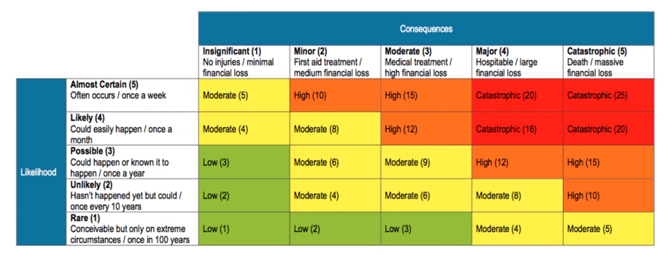
Figure 1: A typical heat map. How well-defined is the difference between a “high financial loss” and a “large financial loss”?
Yet despite the limits to the pseudo-quantitative approach, it is often the basis for setting strategy and budgets with a high level of specificity. This was brought home to us at Protiviti when we recently co-sponsored a survey of 1,300 executives regarding the cybersecurity practices of their organizations. Of the nearly 850 respondents whose firms weren’t using quantitative risk assessment, nearly half said their companies had a less than 10 percent chance of suffering more than $1 million in cyber losses in 2019 — despite the fact that these companies, without quantitative risk assessment, were unlikely to be able to base such a claim on anything more than gut instinct. Call it the “Heat Map Trap.”
The good news is that there is a clear path to implementing a risk assessment program that is authentically quantitative and in which confidence is justified. The first step is to clearly delineate the issue at hand and the possible outcomes. Take, for example, the essential task of evaluating the relative impact of various cybersecurity risks. One such risk might be that of a non-malicious insider clicking on a phishing email that gives an intruder access to financial accounts. That threat scenario is actually a string of several separate events, each of which has a range of probabilities of occurrence and losses attached to it (a distribution).
This deconstruction of larger business questions into their components is the most challenging step in the process — it’s common in first attempts at quantitative modeling to struggle with data and estimates because the scope or scenario hasn’t been properly defined. But these speed bumps are easily overcome with guidance and experience.
Once the models have been developed, they are then populated with the distributions of frequencies and losses associated with each event. These distributions let us account for the level of uncertainty in our estimates, the less sure of the actual value we are the wider the distributions become. We have found that meaningful insights can still be obtained even when we have seemingly large degrees of uncertainty and wider ranges of possible values.
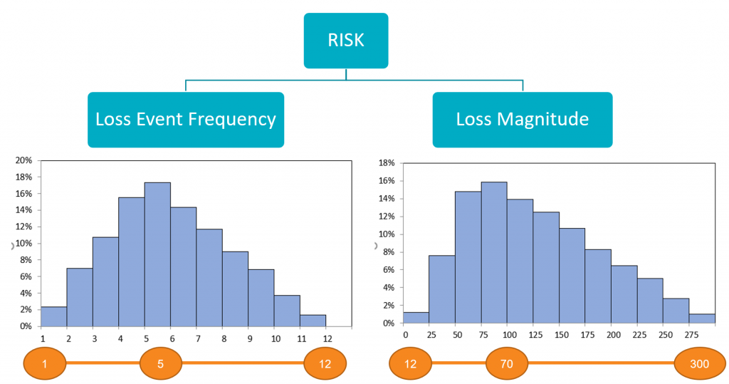
Figure 2: Proper quantitative risk assessment reduces risk to combinations of probabilities and losses.
This is the critical point where the subjectivity of the heat map is replaced by the objectivity of tangible data. It’s also the point at which many people shy away from quantitative risk assessment because they don’t have all (or any of!) the data they need. But it’s a fallacy to think that you have to have perfect data — even imperfect data can provide meaningful estimates that lessen the uncertainty of the analysis. (There are also cybersecurity data sets that have been validated over time that can be used until the enterprise begins to collect its own data.) And remember that we use statistical methods precisely because we don’t have complete information. If we had 100% complete data we wouldn’t need to do an analysis at all.
Once frequencies and loss distributions have been assigned, Monte Carlo simulations generate a probability distribution curve plotting the likelihood of a loss exceeding a certain amount. This gives cyber decision makers a much clearer view of the threats that they are facing and the relative benefits of mitigating those threats — or, to take the question we asked on the survey, the probability of suffering a cybersecurity loss of more than $1 million over the course of a year.
Translating the problems or questions that arise in decision making into probabilities and losses is necessary to make meaningful comparisons of different options. In the hypothetical example below, the orange data shows how addressing certain issues in a system reduces expected losses, allowing for a much more concrete cost-benefit analysis of that plan of action.
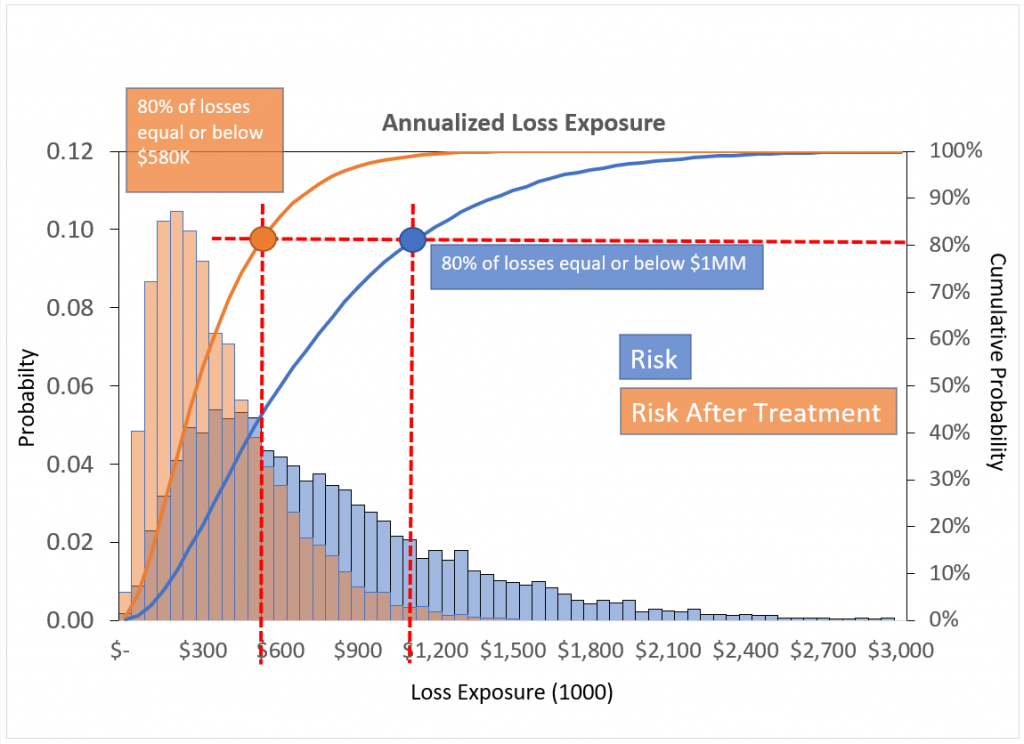
Figure 3: Decision making is easier when you can make direct comparisons between courses of action.
According to our cybersecurity survey, half of the companies that are not currently using quantitative risk assessment expect to do so within the next two years. Most of those firms will find that starting with a clearly defined pilot program is the most convincing way to establish the proof of concept necessary for wider adoption.
Cybersecurity professionals labor in an environment in which little is certain. But even if it is full of shadows, there are definite contours to the landscape. Quantitative risk assessment offers a way of determining the shape of those contours and enabling more confident decision making at a time when every organization finds its cybersecurity function under scrutiny.
Find more posts on The Protiviti View related to cybersecurity.

Thanks for the post. But how will you calculate ALE if Lost Event Frequency is not 1-12 but for example 30% of occurring in the next year? Will you multiply 30% by Loss Magnitude, or will you use Bernoulli distribution for representing of likelihood?
Great question – We would still want to express Loss Event Frequency as a range as there always a level of uncertainty. A 30% chance of occurring essentially means that the event would occur approximately every 3 years. We would just express Loss Event Frequency as a decimal, for example a 30-40% chance of occurring would be expressed as 0.3-0.4.
Feel free to reach out via the contact form if you would like to discuss in more detail.
Thanks,
Vince
Ilya
I would use a Poisson distribution, as there may be more than one event – but apart from that. Yes, the Poisson with a 30% (average) likelihood over one year – and repeated annually for whatever timeframe you are looking at. Then combined with the distribution of losses (which is likely to be something like a lognormal distribution) will give you a result which is precise enough to make decisions on.